This is a brief introduction to neural networks. We will start below by comparing the traditional machine learning pipeline to the neural network pipeline. We will then discuss perceptrons, multiple perceptrons, bias implementation, composition, non-linear activation, and convolution neural networks.

Revised on Jan 3, 2026

---

Here is a common machine learning pipeline. Each bullet lists the manual steps that must be taken to build a classifier. The goal of neural networks is to automate these steps.

1. Image formation - Manually capturing photos for database

2. Filtering - Hand designed gradients and transformation kernels

3. Feature points - Hand designed feature descriptors

4. Dictionary building - Hand designed quantization and compression

5. Classifier - Not hand designed, learned by the model

Goal of Neural Networks: To build a classifier to automatically learn [2-4]

Compositionality: For images, an image is made up of parts, and putting these parts together creates a representation.

Perceptrons

Neural networks are based on biological neural nets.

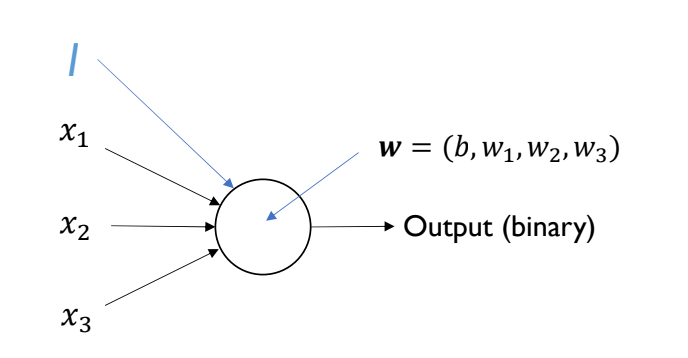
For linear classifiers, we formulate a binary output (classifier) based on a vector of weights $w$ and a bias $b$

$output = \begin{cases} 0 & \text{if } w \cdot x + b \leq 0 \\ 1 & \text{if } w \cdot x + b > 0 \end{cases}$

Example: For a $28\times 28$ pixel image, we can vectorize the image into a $1 \times 784$ matrix. The dimensions of our variables will be:

$x = 1 \times 784$

$w = x^T = 784 \times 1$

$output = xw + b = (1 \times 784) (784 \times 1) + b = (1 \times 1) + b=$ (scalar)

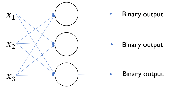
Multiple Perceptrons

For a multi-class classification problem, we can add more perceptrons as above. We then pass in each input value to each perceptron.

Example: For a $28\times 28$ pixel image, we can vectorize the image into a $1 \times 784$ matrix. But now we have 10 classes. The dimensions of our variables will be:

$x = 1 \times 784$

$W = x^T = 784 \times 10$

$b = 1 \times 10$

$output = xW + b = (1 \times 784) (784 \times 1) + 1 \times 10 = 1 \times 10 + 1 \times 10=$ (vector)

Bias implementation

To implement bias, we must add a dimension to each input vector. This input value should be consistent between perceptrons and input vectors, usually just a $1$ at the start or end of a vector. This increased dimensionality, adds a weight to our perceptron, and this extra $w_i$ is the bias, $b$ of the perceptron.

Composition

The goal of composition is to attempt to represent complex functions as a composition of smaller functions. Compositional allows for hierarchical knowledge.

The output vector per perception of one layer must have equal dimension of the input vector to the next perceptron layer.

This is also known as multi-layer perceptron. The perceptron layers between the initial input and final output are known as hidden layers. Usually, deeper composition with more hidden layers gives better performance, and these deeper compositions are known as deep learning.

Non-linear activation

Because our perceptron layers are linear functions, we could reduce these layers to a singular function, which isn’t very helpful. In other works, a multi-layer perceptron neural network (NN) could be simplified to a single-layer perceptron NN if the layers are linear. A non-linear activation function introduces non-linearity to the neural networks.

$$g(x) = f(h(x))$$

We can introduce a non-linear activation function to transform our features.

Example non-linear activation function (Sigmoid):

$$\sigma(z) = \frac{1}{1 + e^{-z}}$$

Rectified Linear Unit (ReLU)

A popular non-linear activation function:

$$f(x) = max(0, x)$$

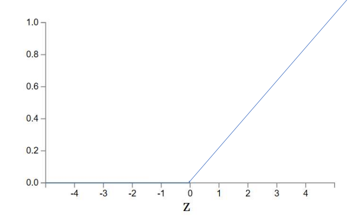
ReLU layers allow for locally linear mapping and solves the vanishing gradients issue. The vanishing gradients issue occurs when gradients dimish while training a deep learing model, and is often dependent on the activation function.

Here is a fun visual for activation functions and hidden layers.

Convolution Neural Networks (CNNs)

It is too computationally expensive to train neural networks on vectorized images. Instead we have to use convolution.

Convolution works by sliding a kernel over an image. For each neuron, it learns its own filter (kernel) and convolve it with the image. The result of this convolution process is a feature map.

$$h[m,n] = \sum f[k,l] I[m +k, n+l]$$

This is known as a convolution neural network. We decide how many filters and layers to train.

This original convolution function $h[m,n]$ is transformed to

$$h_j^n = max(0, \sum_{k=1}^K h_k^{n-1} * w_{kj}^n)$$

where $n=$ layer number, $K=$ kernel size, $j=$ # of channels (input) or filters (depth)

---

Neural Network Layers

This is a brief introduction to different layers in neural networks.

Hidden Layer

A hidden layer is any layer that falls between the input and output layers. Many of the layers we discuss below are hidden layers, as they are neither the input nor the output layer.

The input layer is the first layer of the neural network. It is the layer that receives the input data. The output layer is the final layer of the neural network. It is the layer that produces the output data.

Convolution Layer

A convolution layer is typically used to detect patterns in an input volume. The layer applies a filter to an input volume by sliding a filter over the volume, in a method known as convolution.

Convolution is the mathematical process of applying a filter by sliding it over the input volume. The filter is typically much smaller than the input, and the output volume is reduced in size. For neural nets, the performance difference between convolution and correlation is minimal. In real world applications, correlation is often used under the hood because it is slightly faster to compute than convolution. The only difference between the two is the rotation of the filter ($-180deg$).

An input volume is the input to the convolution layer. It is a volume because not only does it have width and height, but it also has depth. For example, we typically think of images as 2D (width and height), but the RGB channels provide a depth. Even if the input is grayscale, it still has a depth of 1, and may increase depending on the series of convolution layers. Layers are stacked on top of each other and may change the depth of the original input volume.

Pooling Layer

A pooling layer is used to reduce the spatial dimensions of the input volume. Generally, these layers are used to reduce the spatial complexity of the network and reduce computational expense. For a neural network, this reduces the total number of paramaters and computations.

Pooling layers are convolutational layers that reduce the size of the input volume.

Example: Max Pooling

For max pooling, the output value is the maximum value in the filter’s application.

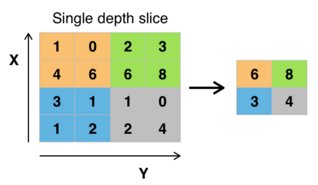
We have a $4 \times 4$ input volume. We apply a $2 \times 2$ filter with a stride of $2$. The output volume is $2 \times 2$.

A filter’s stride is the number of pixels by which the filter shifts over the input volume. Because the stride is $2$ and the filter is $2 \times 2$, there is no overlap in the filter’s application. Generally for pooling layers, the stride is equal to the filter size.

The equation for max pooling is:

which simply defines the sliding for $\text{output} = \max(\text{input})$

Fully Connected Layer

If every neuron in the current layer is connected to every neuron in the previous layer, the layer is known as a fully connected layer. This is the most common type of neural network layer.

A neuron is a single node in a neural network. Neurons are also known as perceptrons in the context of neural networks. It takes in a set of input data, processes it with a set of weights and biases, and produces a set of output data. More information on the neuron (perceptron) can be found here.

Local Response Normalization Layer

Local response normalization is a technique used to normalize the output of a neuron based on the output of neighboring neurons. This is often used in convolutional neural networks.

Normalization is the process of scaling the output of a neuron to a specific range. This can help the network learn more effectively.

There are two main types of local response normalization (LRN):

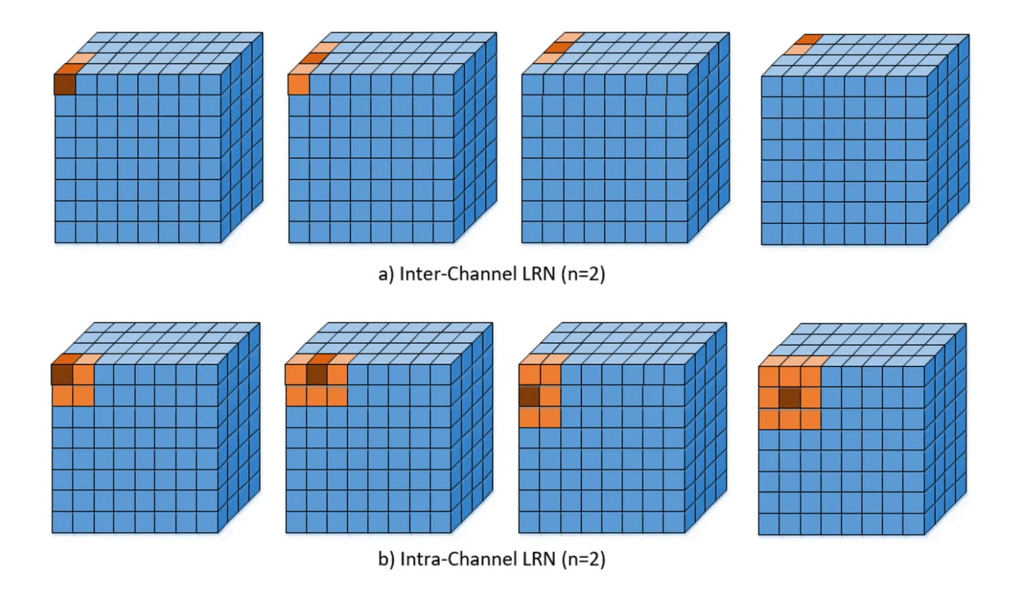
Inter-Channel: Normalize the output based on a 1D slice of the output tensor. This is used in the AlexNet architecture we will see below.

Intra-Channel: Normalize the output based on the output of neighboring neurons in the same channel. This is a 2D slice of the output tensor. This is the more common type of LRN.

A tensor is a fancy term for a multi-dimensional array of numbers. In the context of neural networks, tensors are used to represent the input and output data of the network.

Architecture Diagram

The architecture of a neural network is often represented as a series of layers. We create diagrams of these layers to visualze what is happening between the input and output layers.

Example: The AlexNet architecture. As you’ll see, there are many layers and statistics included in this visualization. I will break them down below.

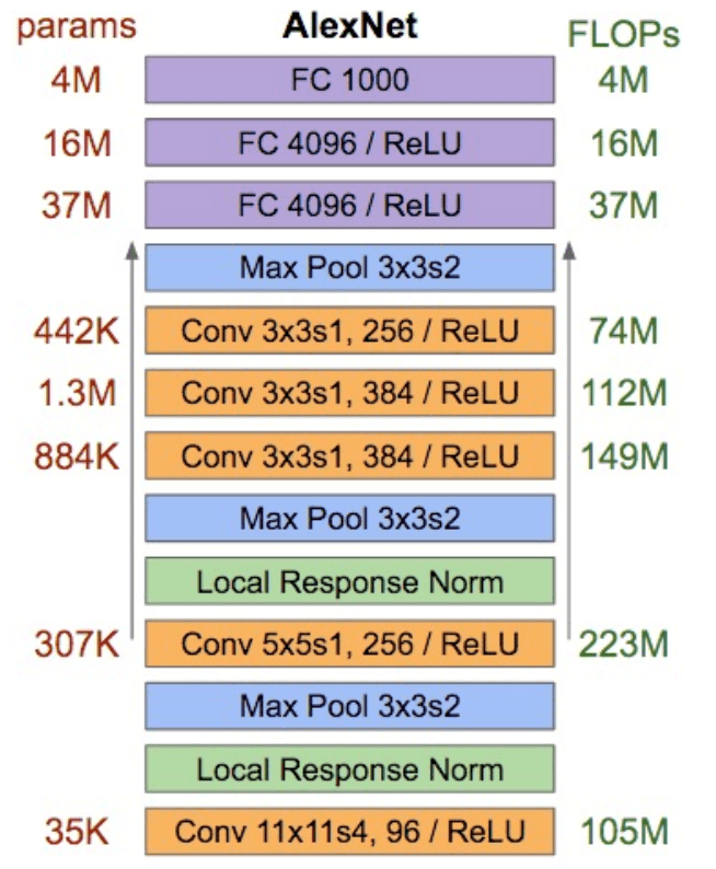
On the left we see params, the number of parameters given to each layer. This is the number of weights and biases in that layer, and the input dimensions.

On the right we see FLOPs, the number of floating point operations. This is the number of operations required to compute the output of the layer.

The blocks in the middle are the individual layers. The layers are going from bottom to top based on the arrow direction on each side of the blocks. These blocks include various information about the layer, including its type, filter dimensions, stride, and

We can visualize the same architecture in a different way:

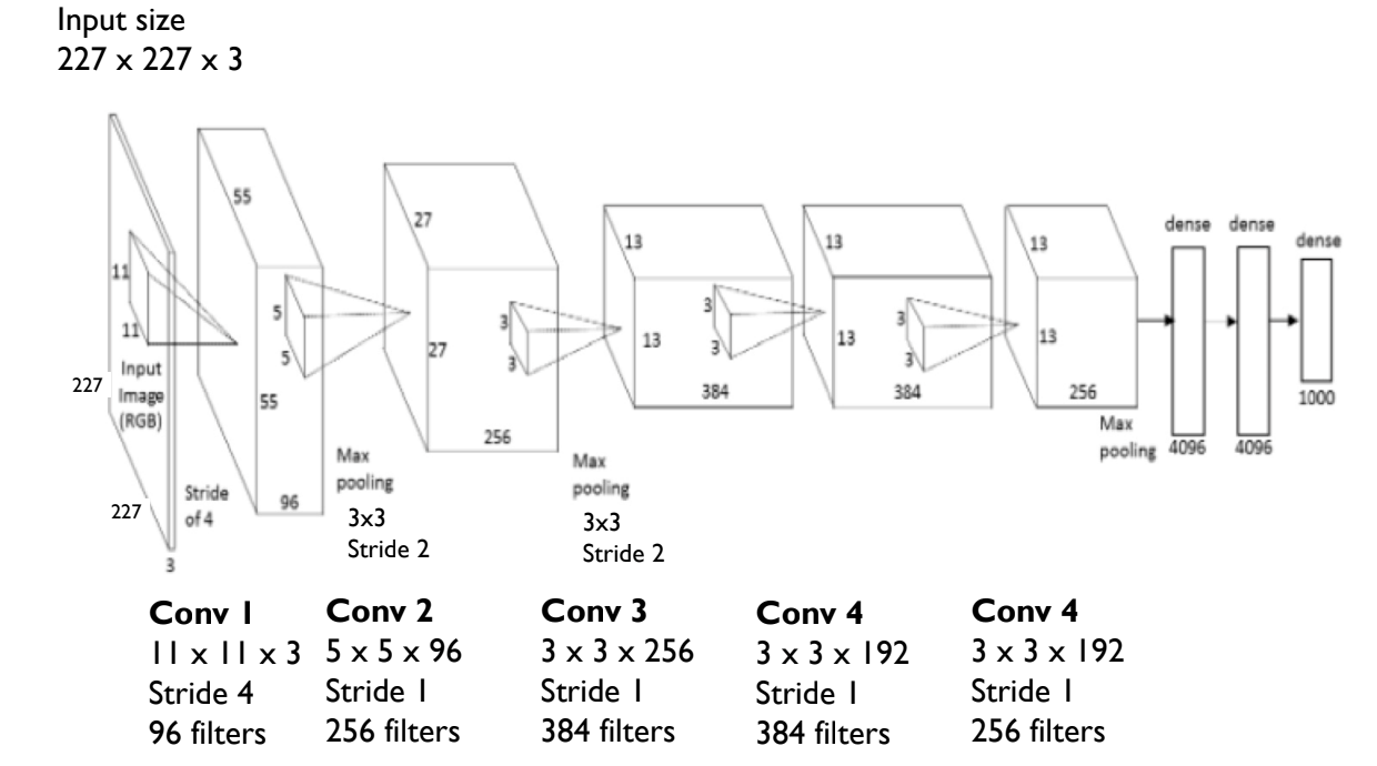
This 3D representation gives us the same information, but in a different format. We can see the input volume, the convolutional layers, and the fully connected layers by relative size.

---

Training Neural Networks

This is a guide to implementing a neural network and training with gradient descent.

Background

We will start with an example identifying handwritten digits using the MNIST dataset. This problem has 10 classes (digits $0-9$). Each image in the database is $28 \times 28$ pixels, meaning each input is a linearlized $1 \times 784$ vector. The output of the CNN will be a $1 \times 10$ vector, where each feature represents the probability of the input being a digit $0-9$.

For now, let’s suppose our network has one fully-connected layer with 10 neurons, one neuron per class or digit. Each neuron has a weight for each input and a bias term.

A neuron is a single node within a neural network layer. Neurons, also known as perceptrons, take in and process a set of data and output a set of data. More information on the neuron (perceptron) can be found here.

Because our first layer is a fully-connected layer, each neuron in this layer takes in all the input data, making 784 connections and weights. More on different neural network layers here.

Definitions

Let’s define variables for our network:

• $x$ is the input data, a $1 \times 784$ vector.

$$x = \begin{bmatrix} x_1 & x_2 & \cdots & x_{784} \end{bmatrix}$$

• $y$ are the input data labels, a $1 \times 10$ vector.

$$y = \begin{bmatrix} y_1 & y_2 & \cdots & y_{10} \end{bmatrix}$$

• $p$ is the probability output of the network, a $1 \times 10$ vector. Each value in $p$ corresponds to a value in $y$.

$$p = \begin{bmatrix} p_1 & p_2 & \cdots & p_{10} \end{bmatrix}$$

• $w$ are the weights per neuron, a $784 \times 1$ matrix per neuron. For all 10 neurons, $w$ is a $784 \times 10$ matrix.

$$w = \begin{bmatrix} w_{1,1} & w_{1,2} & \cdots & w_{1,10} \\ w_{2,1} & w_{2,2} & \cdots & w_{2,10} \\ \vdots & \vdots & \ddots & \vdots \\ w_{784,1} & w_{784,2} & \cdots & w_{784,10} \end{bmatrix}$$

• $b$ are the bias of a neuron. For all 10 neurons, $b$ is a $1 \times 10$ vector.

$$b = \begin{bmatrix} b_1 & b_2 & \cdots & b_{10} \end{bmatrix}$$

• $l$ is the output of the fully-connected layer, a $1 \times 10$ vector. $l$ stands for logits.

$$l = \begin{bmatrix} l_1 & l_2 & \cdots & l_{10} \end{bmatrix}$$

Now we can define an output per neuron in the fully connected layer:

$$l_j = w_j \cdot x + b_j = \sum_{i=1}^{784} w_{i,j} \cdot x_i + b_j$$

where $j$ is the index of the current neuron.

We can turn our logits into probabilities for each class:

$$p_j = \frac{e^{l_j}}{\sum_j e^{l_j}}$$

This is simply the exponential of the current logit divided by the sum of all logit exponentials. This is known as the softmax function.

The softmax function is guarenteed to output a probability distribution ($\sum_j p_j = 1$), and is popular for determining the best class in a classification problem for convolutional neural networks.

To train our model, we want to define a loss function for the difference between $p$ and $y$, our predicted and actual values:

$$L(w,b,x) = -\sum_j^{10} y_j \log(p_j)$$

where $y_j = 1$ if the input is class $j$, and $0$ otherwise.

This is known as the cross-entropy loss function. We can use this loss function to compute error, which is defined as $1 - \text{accuracy}$.

Cross-entropy loss measures how well the predicted probability distribution matches the actual distribution. This loss function minimizes the amounts of information needed to represent the truth distribution versus our predicted distribution. When the amount of information needed is similar, the loss is low and both distributions are similar. There are other loss functions available, but cross-entropy most is popular for classification problems.

Training

To train our model, we calculate the loss function $L$ for every different training example, also known as an epoch. We repeat this for many epochs until hte loss over all training examples is minimized.

A training example is a single input and output pair. This is used to update the weights and biases of the network. An epoch is a single pass through the entire dataset. This is used to update the weights and biases of the network.

The most common strategy for minimizing the loss function is gradient descent. For each training example, we will use backpropagation to update weights and biases via a learning rate.

Gradient descent is an optimization algorithm to minimize a function by iteratively moving in the direction of steepest descent. Steepest descents are calculated by the gradient of the function at the current point.

The learning rate is one of the neural network’s hyperparameters. It determines how far each step of gradient descent should go.

Backpropagation is a method to calculate the gradient of the loss function with respect to the weights and biases of the network. Backpropagation is used with gradient descent to update the weights and biases.

The weights and biases are updated as follows:

$$w_{i,j} = w_{i,j} - \lambda \frac{\partial L}{\partial w_{i,j}}$$ $$b_j = b_j - \lambda \frac{\partial L}{\partial b_j}$$

where $\lambda$ is the scalar learning rate.

In order to calculate the partial derivatives, we need to deduce $\frac{\partial L}{\partial w_{i,j}}$ and $\frac{\partial L}{\partial b_j}$ in terms of $x_i$ and $p_j$.

The derivatives are as follows:

$$\begin{equation} \frac{\delta L}{\delta w_{ij}} = \frac{\delta L}{\delta p_a} \frac{\delta p_a}{\delta l_j} \frac{\delta l_j}{\delta w_{ij}} =\begin{cases} x_i(p_j-1), a = j\\ x_ip_j, a\neq j \end{cases} \end{equation}$$ $$\begin{equation} \frac{\delta L}{\delta b_j} = \frac{\delta L}{\delta p_a} \frac{\delta p_a}{\delta l_j} \frac{\delta l_j}{\delta b_j} =\begin{cases} (p_j-1), a = j\\ p_j, a\neq j \end{cases} \end{equation}$$

We skip much of the calculation here, but the derivatives are derived from the chain rule, using backpropagation. More extensive derivation walkthroughs can be found here.

Sources

• AlexNet
• Computer Vision @ Brown
• Difference between Local Response Normalization and Batch Normalization