This is a brief introduction to different layers in neural networks.

Hidden Layer

A hidden layer is any layer that falls between the input and output layers. Many of the layers we discuss below are hidden layers, as they are neither the input nor the output layer.

The input layer is the first layer of the neural network. It is the layer that receives the input data. The output layer is the final layer of the neural network. It is the layer that produces the output data.

Convolution Layer

A convolution layer is typically used to detect patterns in an input volume. The layer applies a filter to an input volume by sliding a filter over the volume, in a method known as convolution.

Convolution is the mathematical process of applying a filter by sliding it over the input volume. The filter is typically much smaller than the input, and the output volume is reduced in size. For neural nets, the performance difference between convolution and correlation is minimal. In real world applications, correlation is often used under the hood because it is slightly faster to compute than convolution. The only difference between the two is the rotation of the filter ($-180deg$).

An input volume is the input to the convolution layer. It is a volume because not only does it have width and height, but it also has depth. For example, we typically think of images as 2D (width and height), but the RGB channels provide a depth. Even if the input is grayscale, it still has a depth of 1, and may increase depending on the series of convolution layers. Layers are stacked on top of each other and may change the depth of the original input volume.

Pooling Layer

A pooling layer is used to reduce the spatial dimensions of the input volume. Generally, these layers are used to reduce the spatial complexity of the network and reduce computational expense. For a neural network, this reduces the total number of paramaters and computations.

Pooling layers are convolutational layers that reduce the size of the input volume.

Example: Max Pooling

For max pooling, the output value is the maximum value in the filter’s application.

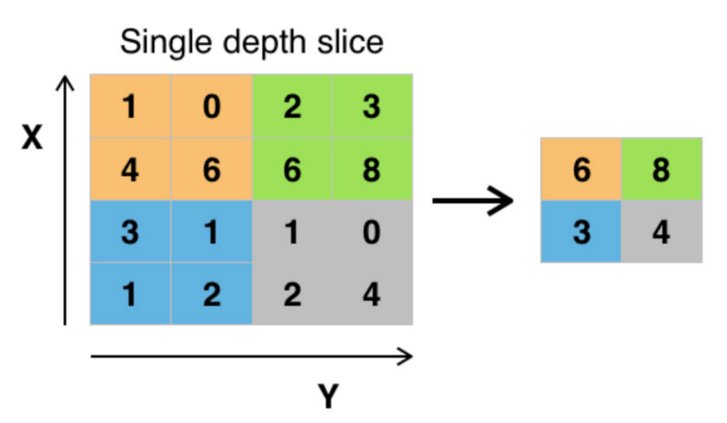
We have a $4 \times 4$ input volume. We apply a $2 \times 2$ filter with a stride of $2$. The output volume is $2 \times 2$.

A filter’s stride is the number of pixels by which the filter shifts over the input volume. Because the stride is $2$ and the filter is $2 \times 2$, there is no overlap in the filter’s application. Generally for pooling layers, the stride is equal to the filter size.

The equation for max pooling is:

which simply defines the sliding for $\text{output} = \max(\text{input})$

Fully Connected Layer

If every neuron in the current layer is connected to every neuron in the previous layer, the layer is known as a fully connected layer. This is the most common type of neural network layer.

A neuron is a single node in a neural network. Neurons are also known as perceptrons in the context of neural networks. It takes in a set of input data, processes it with a set of weights and biases, and produces a set of output data. More information on the neuron (perceptron) can be found here.

Local Response Normalization Layer

Local response normalization is a technique used to normalize the output of a neuron based on the output of neighboring neurons. This is often used in convolutional neural networks.

Normalization is the process of scaling the output of a neuron to a specific range. This can help the network learn more effectively.

There are two main types of local response normalization (LRN):

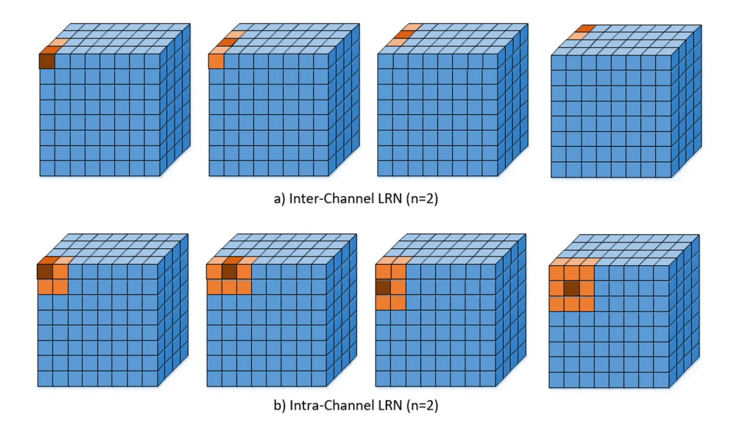
Inter-Channel: Normalize the output based on a 1D slice of the output tensor. This is used in the AlexNet architecture we will see below.

Intra-Channel: Normalize the output based on the output of neighboring neurons in the same channel. This is a 2D slice of the output tensor. This is the more common type of LRN.

A tensor is a fancy term for a multi-dimensional array of numbers. In the context of neural networks, tensors are used to represent the input and output data of the network.

Architecture Diagram

The architecture of a neural network is often represented as a series of layers. We create diagrams of these layers to visualze what is happening between the input and output layers.

Example: The AlexNet architecture. As you’ll see, there are many layers and statistics included in this visualization. I will break them down below.

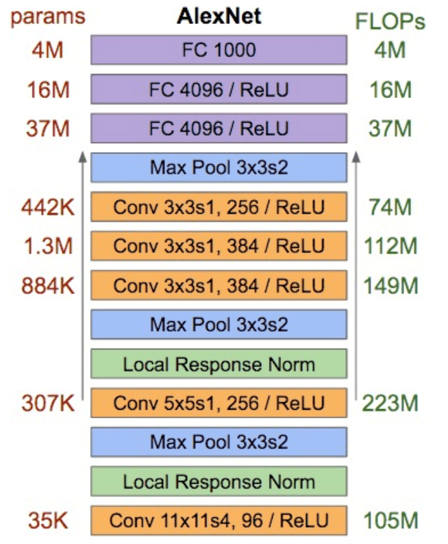
On the left we see params, the number of parameters given to each layer. This is the number of weights and biases in that layer, and the input dimensions.

On the right we see FLOPs, the number of floating point operations. This is the number of operations required to compute the output of the layer.

The blocks in the middle are the individual layers. The layers are going from bottom to top based on the arrow direction on each side of the blocks. These blocks include various information about the layer, including its type, filter dimensions, stride, and

We can visualize the same architecture in a different way:

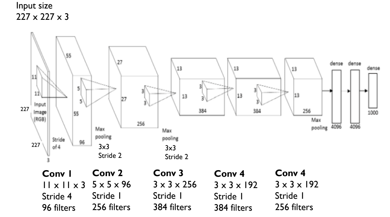
This 3D representation gives us the same information, but in a different format. We can see the input volume, the convolutional layers, and the fully connected layers by relative size.

Sources

• AlexNet
• Computer Vision @ Brown
• Difference between Local Response Normalization and Batch Normalization